My ggplot2 blending adventure
For my sins, I've gone all in on {ggplot2} as my static mapping library within R. Some years ago, I chose a serviceable path for my mapping needs, and then clung to it like my life depends on it, even as many folks I respect extol the benefits of alternative libraries such as {tmap}. That said, there's much fun to be had with {ggplot2} and its myriad extension packages, including {ggforce}, {ggspatial}, {ggh4x}, {ggnewscale}, {ggtext}, {relayer}, {tidyterra} and {ggblend} to name but a few.
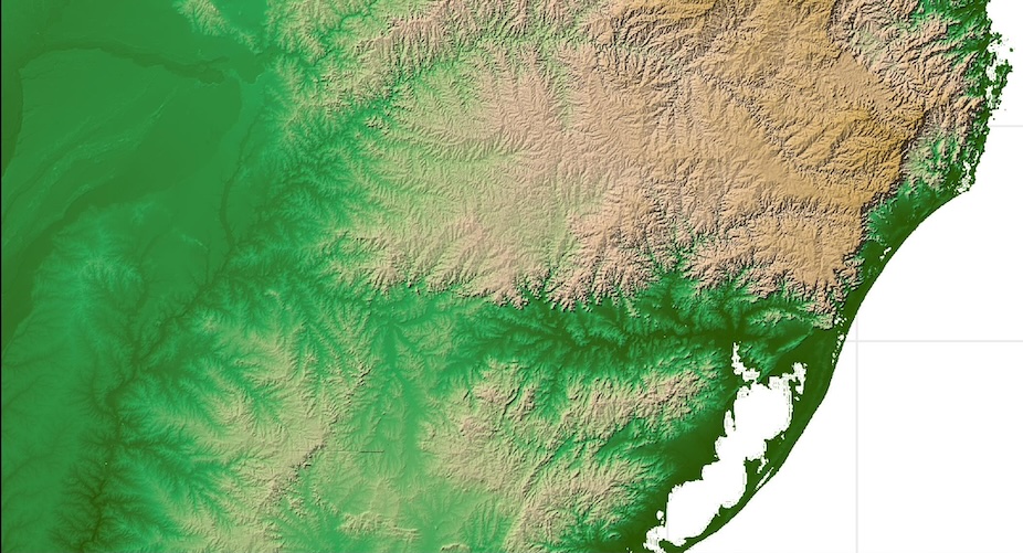
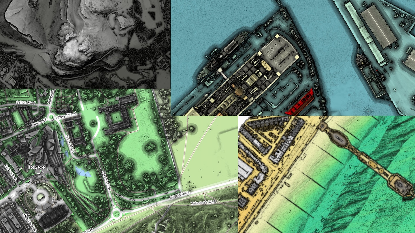
I've also long been a user of the awesome QGIS, which I still turn to for the occassional more cartographic-driven project. This is partly because of one of the great features of QGIS; layer blend modes. These allow the subtle blending of different layers of spatial data using Duff-Porter compositing and blending methods, such as overlay, multiply, and so forth. Employing these techniques, as opposed to (or in combintation with) simple layer transparancy adjustments produces really great looking maps, especially where hillshading is concerned. In fact, one of the talks from last year's FOSS4G:UK was focussed almost exclusivley on how to blend hillshades with various backdrop mapping using suble combinations of layer blend modes within QGIS. The results can be very juicy:
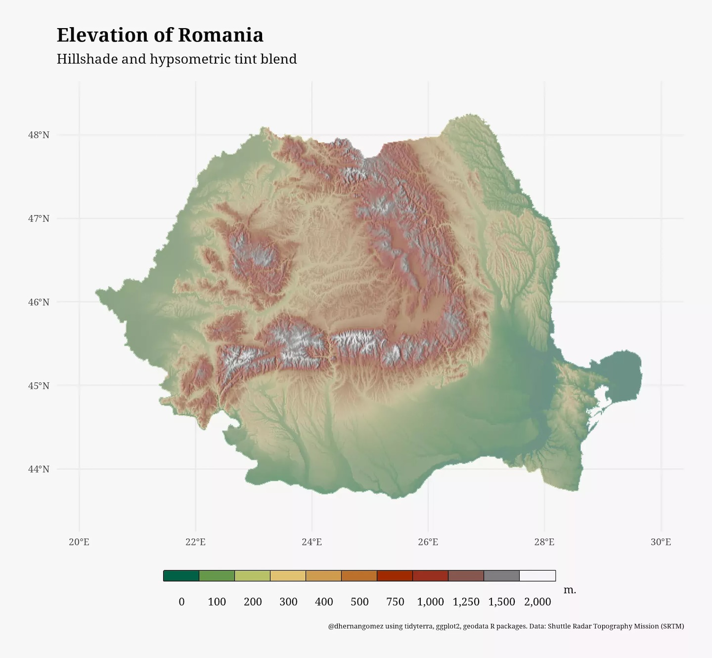
However, I recently discovered that deploying these blend modes whilst plotting spatraster or spatvector spatial data from the terra package in {ggplot2} using {tidyterra} wasn't exactly straightforward. Even this super useful blog post makes no mention of blending, and the final map, whilst awesome in many ways, features an elevation colour palette that looks a bit washed out, because its opacity is set to 40% so that the texture of the underlying hillshade remains visible.
Cue a disproportionately long adventure, involving at least one GitHub issue submission, to figure out how to acheive that polished, QGIS blended look, whilst staying (mostly) within the warm, fuzzy embrace of the R ecosystem. Fortunately, I did eventually discover how to reach this state of nirvana using {ggblend}, though it was hardly pretty. See below for brief summary of journey using SRTM elevation data for southern Brazil. First, we revisit the issue of using just transparency to blend the elevation and hillshade layers:
library(terra)
library(tidyterra)
library(ggplot2)
library(ggblend)

# > r_elev # imported SRTM elevation data
# > r_hs # imported hillshade of SRTM elevation data

# Original plot requires elevation alpha to be reduced so hillshade is visible
maxcell_val <- +Inf

p_alpha_blend <- ggplot() +
    geom_spatraster(
        data = r_hs,
        maxcell = maxcell_val
    ) +
    scale_fill_distiller(
        palette = "Greys",
        na.value = 'transparent',
        guide = 'none'
    ) +
    ggnewscale::new_scale_fill() +
    geom_spatraster(
        data = r_elev,
        maxcell = maxcell_val,
        alpha = .4
    ) +
    scale_fill_hypso_tint_c(
        breaks = c(
            180,
            250,
            500,
            1000,
            1500,
            2000,
            2500,
            3000,
            3500,
            4000
        ),
        na.value = 'transparent',
        name = 'Elevation (masl)',
        guide = guide_coloursteps()
    ) +
    scale_x_continuous(expand = c(0, 0)) +
    scale_y_continuous(expand = c(0, 0)) +
    theme_minimal() +
    theme(panel.border = element_rect(linewidth = 1))

ggsave(
    'tmp.png',
    p_alpha_blend,
    width = 16.5 / 1.25,
    height = 11.7 / 1.25,
    units = 'in'
)
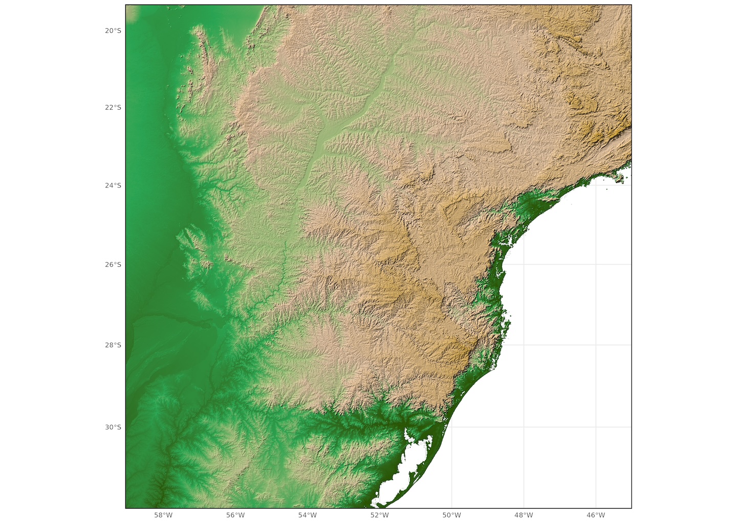
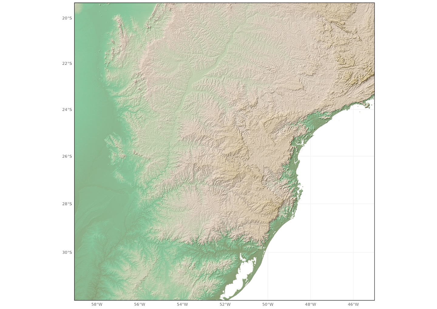 Close, but no cigar. Notice the slightly washed out elevation pallette and lack of definition in the hillshade around lower elevations shown in dark greens
After a failed excursion using {ggfx}, I turned hopefully to the blend() function from {ggblend}. However, the documentation was mainly focussed around blending standard ggplot geom_* calls, with facetting and the like, and there weren't many examples using two completely separate layers with individually defined scales, as in our example. If I tried wrapping the geom_spatraster() and scale_fill_* calls within a list, as recommended, I got an error:
p_mult <- ggplot() +
    list(
        geom_spatraster(
            data = r_elev,
            maxcell = maxcell_val,
            alpha = .4
        ) +
            scale_fill_hypso_tint_c(
                breaks = c(
                    180,
                    250,
                    500,
                    1000,
                    1500,
                    2000,
                    2500,
                    3000,
                    3500,
                    4000
                ),
                na.value = 'transparent',
                name = 'Elevation (masl)',
                guide = guide_coloursteps()
            ),
        geom_spatraster(
            data = r_hs,
            maxcell = maxcell_val
        ) +
            scale_fill_distiller(
                palette = "Greys",
                na.value = 'transparent',
                guide = 'none'
            )
    ) |>
        blend("multiply")


Error:
! Cannot provide both the `object` and `blend` arguments to `blend()` simultaneously.
I momentarily thought I had struck gold after discovering this Github issue, which contained a hacky fix for plotting blended geom_sf() layers. The gist of it was to use the {relayer} package to uniquely name the fill aesthetics for each geom_spatraster() layer, remove the scale_fill_* calls from the list() declaration, and then define them separately per layer after the blend() call. Sadly, this didn't work out for me either.
Finally, after returning to that blog post, a potential fix struck me: what would happen if I set the spatraster geom fills within the geom_spatraster() call itself? To do this, we first need to explicitly define how the raster values map to the geom fill colours, so that we can avoid using the scale_fill_* calls within the plotting pipeline itself and instead set them at a geom level using the fill argument:
# Rename hillshade values
names(r_hs) <- 'shades'

# Generate a grey palette of hex values
pal_greys <- hcl.colors(1000, "Grays")

# Stretch hillshade values across the pallette
index <- r_hs |>
    mutate(
        index_col = scales::rescale(
            shades,
            to = c(1, length(pal_greys)),
            na.rm = F
        )
    ) |>
    mutate(index_col = round(index_col)) |>
    pull(index_col)

# Sample hex values
r_hs_fill <- pal_greys[index]

# Gives character vector of hex values
# > r_hs_fill
#    [1] "#F9F9F9" "#F9F9F9" "#F9F9F9" "#F9F9F9" "#F9F9F9" ...

# We could use a similar approach for the elevation values, using the
# tidyterra::hypso.colors() function to generate the palette.
# However, here I use a different approach to ensure exact
# replication of original palette:

# Create a ggplot2 object using original plotting syntax
r_elev_p <- ggplot() +
    geom_spatraster(
        data = r_elev,
        alpha = 1,
        maxcell = +Inf
    ) +
    scale_fill_hypso_tint_c(
        breaks = c(
            180,
            250,
            500,
            1000,
            1500,
            2000,
            2500,
            3000,
            3500,
            4000
        ),
        guide = 'none',
        name = 'Elevation (masl)'
    )

# Build the plot and extract the colour mapping
g <- ggplot_build(r_elev_p)
r_elev_fill <- g$data[[1]]$fill

# Again, gives character vector of hex values
# > r_elev_fill
#    [1] "#D7E1A2" "#D7E1A2" "#D7E1A1" "#D7E1A1" "#D7E1A1" ...

# Now we can use the list() and blend() syntax expected by {ggblend}
p_multi_blend <- ggplot() +
    list(
        geom_spatraster(data = r_elev, fill = r_elev_fill, maxcell = +Inf),
        geom_spatraster(
            data = r_hs,
            fill = r_hs_fill,
            alpha = .85,
            maxcell = +Inf
        )
    ) |>
        blend("multiply") +
    scale_x_continuous(expand = c(0, 0)) +
    scale_y_continuous(expand = c(0, 0)) +
    theme_minimal() +
    theme(panel.border = element_rect(linewidth = 1))

ggsave(
    'tmp.png',
    p_multi_blend,
    width = 16.5 / 1.25,
    height = 11.7 / 1.25,
    units = 'in'
)
 Much better. The depth and saturation of the original elevation palette is preserved whilst the hillshade remains well defined.
Check below for a side by side comparison!