Getting closer to HPC with R and {targets}

In this post I'll share my own 'low-friction' approach to software development on High Performance Computing (HPC) clusters. I make use of a few different tools for this, including R, {targets} (link), the Python and generalised Conda-like environment manager micromamba (link) and the relativley new, VS Code-alike IDE Positron.
This is more of a tutorial than a simple script or out-of-the-box workflow. I imagine a lot of this will be quite obvious to hardened software developers and engineers and so this post might be most useful to data scientists or computational researchers already familiar with {targets} who want to scale up their analyses to run on HPCs whilst maintaining the feel of developing locally. If you want to follow along, you'll need access to an HPC cluster with SLURM (possible, though not recommended, to set up using AWS), however the general principles should be applicable for different set ups. I'm using MacOSX but the approach should work for most Linux distributions too. Windows users can probably replicate this using the Linux subsystem tool (WSL), though I make no guarantees.
Preamble
I tend to do a lot of my computational research and software development remotely now, thanks in part to a fantastic little bespoke SLURM cluster provided by the kind folks from Bournemouth University Computer Science. Although I really like working on the cluster remotely, like all things in life (other than drinking Aperol spritz and smoking cigarettes in the sun, of course) there are both benefits and drawbacks. The main benefit of this approach is being able to actually develop software and workflows on the 'production' cluster itself, rather than having to constantly push and pull the repo to and from a hosted git instance, which can get tricky with large files and outputs. Ultimately, this makes developing, debugging and running analyses much quicker, however other positives also include:
- Much more disk storage than I could maintain on my laptop (e.g. we have well over 2TB+ per user).
- Much more compute available. The cluster comprises x 6 nodes each with an AMD EPYC 9334 32-Core Processor and ~80GB available RAM. So I can parallelize my computations over 120-192 cores and can access up to 480GB of RAM.
- Remote processing. Using this workflow, I can set my analyses running and then close my laptop or work on other things without having to worry about overloading my local machine or disturbing the analyses.
- (Potential) collaborative opportunities, as theoretically a whole team could work on this repository together (although I've not done this yet)
- Increased portability of projects. Although I could (and should) maintain good computational environment hygiene even when developing on my own laptop, the completely clean environment and lack of root user priviliges on HPCs forces me to always build computing environments from scratch and not assume the existence of any pre-existing software (more on this later).
However the negatives include:
- Online access only, which means I can occasionally be locked out of my work when I don't have internet access.
- Slow connection speeds cause latency issues, rendering interactive sessions somewhat frustrating.
- Variable computing power as shared resources are sometimes not available if other users are running jobs.
- (Potential) increased energy use and thence C02 production–having all that compute at your finger tips makes it easier to crunch a lot of numbers, even when it might not be strictly neccessary.
Getting set up
The first part of this post focusses on configuring Positron for remote working. So go download and install Positron on your local machine. You won't regret it. Next, check OpenSSH is installed by running ssh in your terminal or install it if needed (I believe it is installed as standard in most Linux distributons and on MacOSX).
Now we will configure our local ~/.ssh/config file with details of our SLURM cluster. If the file doesn't already exist then create it using these instructions. We will develop it into something like the below, with different chunks of text defining different hosts. A note: identation (four spaces) and line breaks matter.
Host uni-slurm
    HostName 192.0.0.1
    IdentityFile ~/.ssh/id_ed25519_uni_slurm
    ForwardX11 yes
    User barney

Host uni-slurm-gpu
    HostName 192.0.0.2
    IdentityFile ~/.ssh/id_ed25519_uni_slurm_gpu
    ForwardX11 yes
    User barney
You can define as many hosts as you'd like and do some pretty advanced stuff using this configuration file, however for now we will just focus on the basics. The first line, Host, can be anything you like but best to avoid special characters (some of these are reserved for advanced functionality), excessive spaces etc. The next line HostName is the IP address of your cluster.
The IdentityFile line is key, or I should say, your SSH public key location. Providing this is important as it ensures you can connect to the cluster without typing a password, so follow the below instructions, unless you derive some kind of sick pleasure from repeatedly typing out passwords. We need to generate a key pair (a public and private key) using the ssh-keygen command and then copy the public key to your SLURM cluster. This can be done like so:
# specify the key type using `-t` and the key location using `-f`
ssh-keygen -t ed25519 -f ~/.ssh/id_ed25519_uni_slurm
# choose to add a passphrase or not

# copy to file to the SLURM cluster, supplying the file path and your SLURM username and host address
ssh-copy-id -i ~/.ssh/id_ed25519_uni_slurm barney@192.0.0.1
# enter password to authorize the key
Awesome. You should now be able to SSH into your SLURM cluster without typing your password. Test this out by running ssh uni-slurm (or whatever you named your host) in a terminal and you should be logged in to your SLURM head node with no issues. Fire up Positron and click the Remote explorer button on the left hand side toolbar. You should see your cluster listed under the SSH Targets drop down, click the Connect to Host in New Window button to the right and Positron will first install a little server on to the head node and then connect to it. You might see warnings about no Python or R interpreters being available but don't worry, we will get to that in just a second.
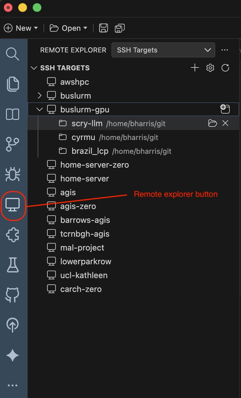
Depending on how your cluster is configured, its unlikely that you will have the correct packages already installed and as a non-root user you won't be able to manually install then using the usual Linux package managers such as apt, yum or dnf etc. You may have the Modules system available, in which case you could load any shared software packages using the module load command but I recommend defining your own computational environments using conda, mamba, micromamba, or even pixi. This helps with reproducibility and generally makes the work more portable. I've not yet used pixi and so, from the conda alike solutions, I rate micromamba the most due to its speed and completely standalone nature (i.e. you won't have to ask your Administrator to install anything). Set up can be a bit fiddly but the installation guide is helpful. You can use the Terminal window shown at the bottom of the screen in Positron to work on the remote cluster directly. If you already have conda or mamba installed then the below instructions should still work.
Once you have micromamba configured, go ahead an create your environment and install the relevant packages using the following:
# create the environment named `foobar` and set the default channel to conda-forge
barney@head:~$ micromamba create -n foobar -c conda-forge

# activate the environment
barney@head:~$ micromamba activate foobar

# install R, targets, tidyverse, crew, and other dependencies
(foobar) barney@head:~$ micromamba install r-base r-targets r-tidyverse r-crew r-crew.cluster r-usethis r-qs2 -c conda-forge
Close and reopen Positron so that it refreshes its list of available interpreters and reconnect to the cluster as before. Now create a new folder for your project: click the New button at the top left of the Positron window and select New Folder from Template, choose R and select an appropriate location on the remote cluster using the same name as your environment (in my case foobar). Select the version of R we just installed using micromamba (the path should be something like .local/share/mamba/envs/foobar, although this may vary). Your session should begin.
At the time of writing, the integration of Positron and R installed within conda/mamba environments is not perfect and it seems that the R session running within Positron does not respect all of the system environment variables that are set when running R directly from an activated conda/mamba environment in the terminal. The problem may be further exasperated by the fact that parallel processing relies on multiple versions of R spawned as subprocesses from the main R session, which again themselves seem to lack key environment variables required for R to function properly. We can fix this by creating a new R file in the project root directory called generate_renviron.R containing the following code (note: do not run this from the R console in Positron):
# One-off script to be run using conda/mamba version of R
# Generates .Renviron file with conda/mamba system environment variables
# Ensures R subprocesses launched by crew have appropriate system variables
env_vars <- Sys.getenv()
conda_env_vars <- base::grepl('^CONDA', names(env_vars))
conda_env_vars_lines <- paste0(
  names(env_vars)[c(conda_env_vars)],
  '=',
  env_vars[c(conda_env_vars)]
)
r_env_vars <- base::grepl('^R_', names(env_vars))
r_env_vars_lines <- paste0(
  names(env_vars)[c(r_env_vars)],
  '=',
  env_vars[c(r_env_vars)]
)

path_lines <- paste0('PATH=', Sys.getenv('PATH'))
cat(
  c(conda_env_vars_lines, r_env_vars_lines, path_lines),
  sep = '\n',
  file = '.Renviron'
)
Now we run this script from our activated environment at the terminal:
# enter the project directory
barney@head:~$ cd ~/git/foobar

# activate the environment
barney@head:~/git/foobar$ micromamba activate foobar

# run R script using `Rscript` command
(foobar) barney@head:~/git/foobar$ Rscript generate_renviron.R
All being well, you should see a file pop up in the project root directory named .Renviron. I won't go over its contents but essentially this file ensures any and all R processes run by the analyses inherit the correct system variables.
Choosing your {targets}
We are now ready to configure {targets} by typing the following command in the Positron console: targets::use_targets(). This will create the various files and folders required by {targets}. I won't get into the details of using {targets}, other than to say it really is worth the time investment. It's an absolute game changer in terms of reproducibility, coding efficiency and computational efficiency. If you want a gentle, expertly delivered introduction and rationale then watch this amazing R-ladies presentation by Irena Papst and check out the official getting started guide. For now, we will define a minimal project with some toy functions and targets. Load up _targets.R and adjust the upper section (i.e. the section above the list of targets) so it matches the below:
# Load packages required for targets script
library(targets)
library(crew)
library(crew.cluster)

# Detect / set free compute nodes
num_idle_workers <- as.integer(system('sinfo -h -t idle -o "%D"', intern = T))
message(paste0('SLURM nodes available: ', num_idle_workers))
if (num_idle_workers == 0) {
  warning('No compute nodes available')
}

# Create / clear logs directory
if (!dir.exists('logs')) { dir.create('logs') }
file.remove(list.files('logs', full.names = T))

# Set target options:
targets::tar_option_set(
  packages = c('tidyverse'),
  format = "qs",
  controller = crew_controller_slurm(
    crashes_max = 2,
    workers = 4, # or can set to all avaialable using `num_idle_workers`
    seconds_idle = 120,
    options_cluster = crew_options_slurm(
      cpus_per_task = 20,
      log_output = "logs/crew_log_o_%A.txt",
      log_error = "logs/crew_log_e_%A.txt",
      memory_gigabytes_per_cpu = (80 / 20)
    )
  )
)

# Toy function that sleeps for 10 seconds and prints a series of numbers and
# system and process info
sleep_and_paste_info <- function(data_split, tar_name) {
  runtime <- Sys.time()
  pid <- Sys.getpid()
  Sys.sleep(10)
  tibble::tibble(
    tar_name = tar_name,
    nums = min(data_split),
    start_time = runtime,
    end_time = Sys.time(),
    pid = pid
  ) |>
    mutate(
      time_diff = end_time - start_time
    )
}
A few customisations are included in this script: i) the addition of a logging mechanism; ii) automatic compute worker detection and; iii) the addition of the {crew} SLURM controller. You can see the various arguments pertaining to the cluster contained within the crew_controller_slurm() and crew_options_slurm() calls. Obviously, you can customise these as needed but for now I've set up a workflow that uses 4 compute nodes each with 20 cores (cpus_per_task = 20), but you can set the number of nodes to as many as are idle at runtime (workers = num_idle_workers). In some ways this is the safer option as if there aren't as many free nodes as requested the pipeline will just hang. For each node I've assigned 80GB of RAM by dividing the total RAM available by the number of cores (memory_gigabytes_per_cpu = (80 / 20)). Now let's move on to defining some targets for our analysis in the lower part of the _targets.R script.
# list of targets to run
list(
  tar_target(
    name = data_split,
    command = list(
      1:25,
      26:50,
      51:75,
      76:100
    ),
    deployment = 'main',
    iteration = 'list'
  ),
  tar_target(
    name = data_split_main_branched,
    command = sleep_and_paste_info(data_split, 'data_split_main_branched'),
    deployment = 'main',
    pattern = map(data_split),
    cue = tar_cue('always')
  ),
  tar_target(
    name = data_split_worker_branched,
    command = sleep_and_paste_info(data_split, 'data_split_worker_branched'),
    deployment = 'worker',
    pattern = map(data_split),
    cue = tar_cue('always')
  ),
  tar_target(
    name = combine_data,
    command = {
      bind_rows(
        data_split_main_branched,
        data_split_worker_branched
      )
    },
    deployment = 'main',
    cue = tar_cue('always')
  ),
  tar_target(
    name = summarise_data,
    command = {
      combine_data |>
        dplyr::group_by(tar_name) |>
        summarise(
          min_start_less_max_end = max(end_time) -
            min(start_time)
        )
    },
    deployment = 'main',
    cue = tar_cue('always')
  )
)
Here, I've used the first target, data_split, to define a list of length four containing toy data, which we then process using the function sleep_and_paste_info() across two subsequent targets using a couple of different distributed configurations, controlled by the target deployment argument. Targets with deployment = 'main', such as data_split_main_branched, are processed using the main R process (i.e. the one running on the cluster head node) and thus should be restricted to minimally demanding tasks, such as loading data. The benefit of this is that you can debug these targets more easily. Targets with deployment = 'worker', such as data_split_worker_branched, are run on the compute nodes.
A key part of the distributed targets workflow is the use of branching, which is facilitated by the pattern = map(data_split) argument, which instructs the parent target to iterate over the child elements of the given target data_split, with separate iterations being assigned to different workers, as required. This is the simplest form of distributed computing using {targets}, Hopefully you can see the possibilities here, with the ability to shunt different targets around our cluster workers as and when (or if) required. Let's run the pipeline by calling targets::tar_make() in the console.
| tar_name | nums | start_time | end_time | pid | time_diff |
|---|---|---|---|---|---|
| data_split_main_branched | 1 | 2026-04-21 11:16:41 | 2026-04-21 11:16:51 | 3884094 | 10.00510 secs |
| data_split_main_branched | 26 | 2026-04-21 11:16:52 | 2026-04-21 11:17:02 | 3884094 | 10.01076 secs |
| data_split_main_branched | 51 | 2026-04-21 11:17:02 | 2026-04-21 11:17:12 | 3884094 | 10.01065 secs |
| data_split_main_branched | 76 | 2026-04-21 11:17:12 | 2026-04-21 11:17:22 | 3884094 | 10.01080 secs |
| data_split_worker_branched | 1 | 2026-04-21 11:17:24 | 2026-04-21 11:17:34 | 72149 | 10.01167 secs |
| data_split_worker_branched | 26 | 2026-04-21 11:17:32 | 2026-04-21 11:17:42 | 72299 | 10.01159 secs |
| data_split_worker_branched | 51 | 2026-04-21 11:17:24 | 2026-04-21 11:17:34 | 73114 | 10.01167 secs |
| data_split_worker_branched | 76 | 2026-04-21 11:17:34 | 2026-04-21 11:17:44 | 72149 | 10.01100 secs |
Assuming the pipeline runs OK, we can now inspect the output by calling targets::tar_read(combine_data), and examining the resulting tibble, as shown above. You can see that the first four rows pertain to the target deployed to the main R process (PID: 3884094). As expected, each of our four toy datasets is processed sequentially by the same R process, with an interval of c. 10 seconds between each iteration's timestamp. The following rows show how the data_split_worker_branched target was processed, with three unique R subprocesses handling the processing of the four toy datasets. We can see the execution times of a couple of these branches are close to simultaneous. Under the hood, {crew.cluster} has written and submitted several SLURM job requests to handle the distribution of each toy dataset iteration across the cluster. If we look at the results of the summarise_data target we can see that the overall clock time of this target is around half that of the target executed using a single R process on the headnode:
| tar_name | min_start_less_max_end |
|---|---|
| data_split_main_branched | 40.15207 secs |
| data_split_worker_branched | 20.09888 secs |
Working this way, you can now further develop your analytical pipeline within Positron, almost as if you were working locally–neat! This is really just the beginning of what you can do with {targets} and {crew.cluster}, which has the functionality to define different groups of workers and functions for interfacing with different HPC architectures, such as Oracle Sun Grid Engine or IBM Spectrum LSF.